lml-example

Example with LML

To introduce LML and its functionality, a few examples are used in the following section. With LML a set of graphical components can be defined. These components are deduced from graphical components of LLview. A summary of LLview's graphical components is listed here. For each component of LLview LML provides a class of XML-tags, which allow the definition of all information needed to generate the associated graphical output. In this section you will find examples for a subset of these graphical components and corresponding LML-source, which contains all information to generate the graphical output.

LML-description of a table

As depicted in the picture below, LLview presents for example important information of running jobs in a table:

graphical output of a job-list as a cut-out of LLview

The LML-Schema defines an XML-tag, which allows to collect all information the table contains. The LML-description is a logical description, which can be easily converted into graphical output. The following LML-Code can be used to describe a table, whose output might be similar to the picture above:

<table title="joblist" id="llviewjoblist">
        <!-- column definitions -->
        <column id="1" name="CPUs" sort="numeric" />
        <column id="2" name="Userid" sort="alpha" />
        <column id="3" name="cpuh" sort="alpha" />
        <column id="4" name="wall" sort="alpha" />
        <column id="5" name="U" sort="alpha" />
        <column id="6" name="Class" sort="alpha" />
        <column id="7" name="Spec" sort="alpha" />
        <column id="8" name="TEnd" sort="alpha" />
        
        <!-- content of table, first row -->
        <row oid="j1">
            <cell value="128" />
            <cell value="User#015" />
            <cell value="13.3h of" />
            <cell value="23:59" />
            <cell value="U" />
            <cell value="m_long" />
            <cell value="n04.p32.t01" />
            <cell value="+02:48" />
        </row>        

</table>

LML-source for a table

This is an example for one table-instance. Every table consists of column- and row-definitions. In this case eight columns are defined. In addition to the column names (attribute "name" within column-tag) you can define a sorting type, which specifies how the data of the corresponding column should be ordered. For instance the values of column "CPUs" are numerical values and therefore they have to be sorted in a different way than all other columns of this table. For the attribute "sort" the values "numeric", "alpha" and "date" are allowed. Thus a column's content can be ordered as numeric, alpha numeric and date values.

This table description is comparable with the description of a table in HTML. However, the XML-tag of LML is specifically designed for tables, which can be found in LLview's output. The tag contains all information needed to create the graphical output shown above. This example demonstrates that LML provides logical descriptions of status information instead of descriptions, which can be directly converted into graphics. The graphical output above is only one possible realization for this LML-source. So LML does not describe how the data must be displayed, but only which data.

Moreover, a LML-tag for one component -- like this tag for a table -- can appear almost indepently from other components. When generating LML-files one is free to leave components out, which are currently not necessary. A LML-file is a combination of descriptions for graphical components like the table in this example. Putting all components together will lead to a graphical output close to LLview's output.

LML-description of a nodedisplay

More interesting than defining a table in LML is the way the nodedisplay of LLview can be described with LML. The nodedisplay of LLview shows the physical status of the observed system. It contains rectangles for each CPU or for groups of CPUs in large systems. These rectangles are coloured in order to identify the job, which is currently running on this CPU. A possible output of this nodedisplay is the following:

graphical output of a nodedisplay showing the parallel computer JUGENE

This image shows a status of the parallel computer JUGENE, which is administrated by Jülich Supercomputing Centre. On the one hand the nodedisplay provides an overview of the physical structure of the parallel computer. On the other hand one can see the connection between CPUs and jobs, which are currently running on the system. Jobs are identified by their color. For instance the first two rows (coloured in red) are completely used by one job. For more information about the nodedisplay of LLview see the nodedisplay-documentation of LLview.

How can LML provide all information needed to create this graphical output by using XML? It is important to allow a flexible way of description as LML should not only be used to describe JUGENE but in best case any parallel computer. The following LML-example can result in the graphical output of a nodedisplay as depicted above:

<nodedisplay title="JUGENE Nodedisplay" id="jugene">
        <!-- definition of empty system -->
        <scheme>
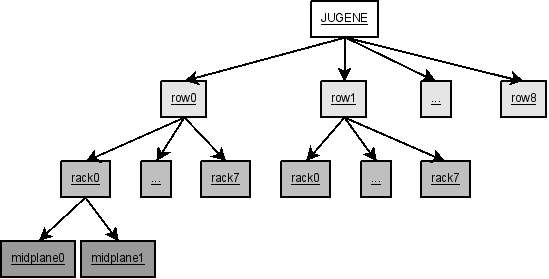
            <el1 tagname="row" min="0" max="8" mask="R%01d">
                <el2 tagname="rack" min="0" max="7" mask="%01d">
                    <el3 tagname="midplane" min="0" max="1" mask="-M%1d">
                        <el4 tagname="nodecard" min="0" max="15" mask="-N%02d">
                            <el5 tagname="computecard" min="4" max="35" mask="-C%02d">
                                <el6 tagname="core" min="0" max="3" mask="-%01d">
                                </el6>
                            </el5>
                        </el4>
                    </el3>
                </el2>
            </el1>
        </scheme>
        <!--  connection between physical elements and jobs -->
        <data>
            <el1 min="0" max="1" oid="job1" />
            <el1 min="2" oid="job2">
                <el2 list="3,5" oid="job3" />
            </el1>
            <el1 list="3,5" oid="job4">
                <el2 list="0,7" oid="job5" />
            </el1>
            <el1 list="4" oid="job6">
                <el2 list="6" oid="job6"/>
            </el1>
            <el1 min="6" oid="job9">
                <el2 list="1,7" oid="job10" />
                <el2 list="3,4,5" oid="job11" />
            </el1>
            <el1 list="7" oid="job12" >
                <el2 min="0" max="3" oid="empty"/>
            </el1>
            <el1 list="8" oid="job13">
                <el2 min="0" max="2" oid="job14" />
                <el2 min="3" max="5" oid="job15" />
                <el2 min="7" oid="empty">
                    <el3 list="1" oid="empty">
                            <el4 min="0" max="3" oid="job7" />
                            <el4 min="4" oid="job8" />
                    </el3>
                </el2>
            </el1>
        </data>
</nodedisplay>

LML-source for status of JUGENE

The nodedisplay-tag consists of two parts: scheme and data.

scheme-tag

The scheme-tag is used to define the system's physical structure. It defines the structure of the empty system. Here, the scheme-tag defines that the parallel computer consists of 9 rows by this line:

<el1 tagname="row" min="0" max="8" mask="R%01d">

Every row contains 8 racks, every rack 2 midplanes and so on. With this scheme-definition it is defined, that the system has 9 rows and because every row has 8 racks, the system has 9*8=72 racks. As a result the system's physical structure is defined by nesting physical elements into each other till the smallest physical element is reached (here core). Therefore a tree of physical elements is build up. The attributes min and max allow to define how many elements of the current type are nested.
This scheme-tag defines a tree with the following structure:

physical structure of JUGENE defined by scheme-tag

The scheme-tag allows to describe this tree very compactly. An advantage of this system-description is its flexibility. The user is enabled to define physical elements arbitrarily. You are not bound to stamp the parallel computer you want to describe into a static tree of nodes and CPUs. The different levels of the tree or in other words the types of physical elements, which are nested, can differ for each parallel computer described with LML.

With the scheme we have a description of the physical structure of an empty system.

The mask-attribute is used to assign distinct names to all physical elements. On each level of the hierarchy the physical elements like rows, racks or midplanes are identified by their ids. On the first level rows are defined with ids from 0 to 8. To generate corresponding names for these rows one could use the C-function "printf". The format-parameter is the mask-value and the only object printed is one of the ids. For the first row (id=0) the printf-call is the following:

printf("R%01d", 0 );

Consequently the names of all rows in this example are "R0", "R1", ..., "R8". For physical elements in lower levels the names of each level are concatenated. For instance midplane0 in rack7 in row3 is identified by the name "printf( "R%01d%01d-M%1d", 3, 7, 0)", which is "R37-M0".

data-tag

The data-tag is needed to connect the physical elements defined by the scheme-tag with jobs running on the system. The data-tag's content refers to the tree-structure given by the scheme-tag. The first line below the data-tag's beginning

<el1 min="0" max="1" oid="job1" />

defines that "job1" is running on rows 0 and 1. In the picture of the nodedisplay row0 and row1 are the first rows on the top of the picture. The rectangles, representing the nodecards of the LML-description, are coloured red for job1. As can be seen the tree created by the data-tag can be collapsed. You can stop describing lower levels, if the oid-definition of the upper level is the same for all elements within this subtree. If you have different jobs running within one subtree, you have to specify the lower-level elements. Therefore you have to expand the tree till you have reached a level where all elements are connected to the same job. If you wanted to define an empty system, you could define the following data-tag:

<data>
    <el1 min="0" max="8" oid="empty"/>
</data>

This means all rows and all racks within these rows and all other lower elements are empty or idle. The values of oid are inherited to all lower elements. With this information, you can understand the following definition of the LML-description of JUGENE's nodedisplay for row2:

<el1 min="2" oid="job2">
       <el2 list="3,5" oid="job3" />
</el1>

First of all it is defined that the whole row2 is used by "job2". This information is inherited to all racks. But row2 contains two racks, which execute job3. These exceptions have to be defined in the lower-level-definitions. Definitions in lower levels overwrite the inherited values. This LML-source defines that rack3 and rack5 within row2 execute job3. Instead of the use of min and max-attributes, which describes coherent lists of physical elements, you can use the list-attribute. Here you can set a list of ids of physical elements, which do not have to be coherent.

The result of this idea is a tree, which is expanded as much as needed. If there is redundant information, it can be compressed in two ways:
1) values of upper levels are inherited to lower levels
2) lists of physical elements can be created, if the structure of the subtrees is identical

The inheritance of values is only possible, because the main structure of the system is defined by the scheme. Without the scheme you would have to expand the tree in the data-tag till the lowest level (here core), because otherwise the existance of physical elements would become unknown.